
Abstract
Data Mining is a process of exploring against large data to find patterns in decision-making. One of the techniques in decision-making is classification. Data classification is a form of data analysis used to extract models describing important data classes. There are many classification algorithms. Each classifier encompasses some algorithms in order to classify object into predefined classes. Decision Tree is one such important technique, which builds a tree structure by incrementally breaking down the datasets in smaller subsets. Decision Trees can be implemented by using popular algorithms such as ID3, C4.5 and CART etc. The present study considers ID3 and C4.5 algorithms to build a decision tree by using the “entropy” and “information gain” measures that are the basics components behind the construction of a classifier model
Author Contributions
Academic Editor: Erfan Babaee, Mazandaran University of Science and Technology, Iran.
Checked for plagiarism: Yes
Review by: Single-blind
Copyright © 2020 Youssef Fakir, et al.
 This is an open-access article distributed under the terms of the Creative Commons Attribution License, which permits unrestricted use, distribution, and reproduction in any medium, provided the original author and source are credited.
Competing interests
The authors have declared that no competing interests exist.
Citation:
Introduction
The decision tree builds a model based on a data set called training data. This set of training data is only a set of records or objects, and each object (record) is characterized by a set of attributes and other special attribute called class label. If the training data has big number of records and small number of noisy data, then the generated model will be well designed, and constructed, otherwise the model will be poorly predicting future unseen records. Since the training data is important, the test data is also important. It is a set of records with unknown label class, used as a validator of the model.
The generated model used as a descriptive or predictive modeling, the descriptive modeling serve to describe the set of attributes that essentially make an object belong to a class or another class. The model shows the priority of each attribute, which influences the belonging of an object to a specific class. The predictive modeling act as a function takes a new object as input, and produces a class that will be attached to that object.
In the next section, we will discuss in depth the measures behind the constructing of the model, then later we will present how to make these measures work with learning algorithms ID31, 2 and C4.53, 4, 5, 6.
Impurity Measure
There several indices to measure degree of umpurity quantitatively. Most of well know indices are entropy, Gini index and classification error. Entropy in simple terms is the measure of disorder in a group of multiple objects 7. Consider the example in Figure 1, with seven triangles, and five circles.
Figure 1.Example for entropy measure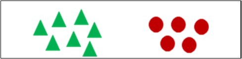
In this example, we cannot be certain of the shape that dominates in totality, this uncertainty we can express it mathematically by the following expression:

where n is the number of classes, and pi is the fraction of an object i by the total number of objects.
Taking the previous example, we get:

The entropy value is between zero and one, its value for the previous example is very high, which means high disorder. Thus, the set of objects is heterogeneous.
We will take another two more examples to illustrate the relations between disorder and the entropy value. The process is the same. Calculate the entropy value for each example.
In this example (Figure 2), we take six green triangles, and two red circles, then calculate again the entropy value for this case:
Figure 2.Example for illustrating the relation between disorder and the entropy

As we see here the value of entropy become smaller, because the group of triangles have much more members than group of circles, which means that the disorder becomes smaller.
In this last example (Figure 3), only take only a set of triangles as describe below:
Figure 3.Example for illustrating the relation between disorder and the entropy

The entropy value indicates that there is no disorder, and that the hole is homogenous. To conclude when a group of objects of different class, or a set of data is heterogonous, the disorder is very high then the entropy value is also high, otherwise when there is homogeneity among a set of data then the entropy value is zero.
There are other measures of impurity 2, such as “Gini Index”, that measures the divergence between the distributions of the target attribute’s values and the “classification error”:


Earlier we see what impurity is. The next step is to find out what information gain is and how it relates to impurity.
Information Gain Measure
Information gain is a measure which makes it possible to discover, among all attributes which characterize a set of records or objects, the attribute that return enormous information about these records. In other words, the attribute that return the lowest impurity 7.
If we have a parent node composed of several objects, each object has several attributes and a class label. We can partition the parent node into sub-set using an attribute. The goal is to discover the attribute that partitions the parent node of objects or records into sub-sets, with the following constraint, each sub-set must be the purest set possible. Means that the sub-set must has a low impurity value.
Information gain is mathematically defined as:

Where I(*) is the impurity measure of a node, we can calculate it by one of the tree measured defined in the impurity section. N is the total number of records or objects in the parent node or parent set, k is the number of attribute values, and N(vj) is the number of records associated with the sub-set vj. Here is an illustrative example of computing information gain measure for different attributes on set of objects, there are twelve object in total, each object represents a person, in general each person characterized by a set of attributes like age, eye color, family status, name, weight…etc. However, in our case, we will take only two attributes (age and weight), and the class label (gender) which only takes two possible values (male or female). Male is represented by triangles, and female represented by circles, as described in the Figure 4. There are seven male and fourth female:
Figure 4.Example of gender illustrating
The impurity for this parent node is equal to 0.979. The impurity is enormous and it makes sense because the set of objects is heterogonous. The main objective is to reduce this impurity. The solution consists in dividing this parent node into sub-set by each attribute from this list of attributes (weight, age), and calculate for each attribute the information gain. Then take the attribute that returns the largest information gain measure.
· Dividing the parent set by the “Weight” attribute.
The weight attribute has three possible values (Figure 5), small, medium and large, this attribute divides the parent set into three sub-sets, a set for small people, contains a male and two female, a set for medium people, contains, two male and a female, and last sub set for large people contains, four male and a female.
Figure 5.Attribute values


Calculate the Information Gain
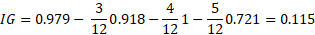
When we divide the parent set by the weigh attribute, the information gain gives the value 0.115.
· Dividing the parent set by the “Age” attribute.
The age attribute also has two possible values, young and adult. The young value gives a sub-set, with three male and two female, and the adult value gives sub-set, with four male and three female (Figure 6).
Figure 6.Attribute values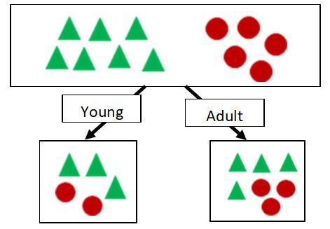


Calculate the Information Gain

The information gain provided by the weight attribute is very high compared to the other age attribute, and the subsets provided by the weight attribute are purer than the subsets provided by the age attribute. Therefore, for this initial parent node, we will take the weight attribute to divide the initial parent node into purer subsets.
(Table 1)
Table 1. Information gain| Weight | Age | |
| Information Gain | 0.115 | 0.00025 |
What is the use of this information gain measure in the classification process? Moreover, how can it be used in the decision tree classifier to construct a model?
These questions will be answered in details in the next section.
The Core of Decision Tree Algorithms
Decision tree algorithms use an initial training data set characterized by a dimension (mXn), m designed to the number of rows in the training data set, and n designed to the number of attributes that belongs to a record. The decision tree algorithms run through that search space recursively, this method called tree growing, during each recursive step, the tree growing process must select an attribute test condition to divide the records into smaller subsets. To implement this step, the algorithm used the measure of the information gain that we saw previously. This means that the decision tree algorithms calculate the information gain for each attribute and this process called the attribute test condition, and choose the attribute test condition that maximize the gain. Then a child node is created for each outcome of the attribute test condition and the sub records are distributed to the children node based on the outcomes. The tree growing process repeated recursively to each child node until all the records in a set belongs to the same class or all the records have identical attribute values. Although both condition are sufficient to stop any decision tree algorithm.
The core and basis of many existing decision tree algorithm such as ID3, C4.5 and CART is the Hunt’s algorithm 11. In Hunt’s algorithm, a decision tree is grown in a recursive way by partitioning the training records into successively purer data set. A skelton for this algorithm called “TreeCrowth” is shown below. The input to this algorithm consists of the training record E and the list of attributes F.
TreeGrowth(E,F)
1) If stropping_condition (E,F) = true then
2) Leaf_node = createNode()
3) Leaf_node = classify()
4) return leaf_node
5) Else
6) root = createNode()
7) root_test_condition = findBestSplit(E,F)
8) let V = {v | v is a possible outcome of root_test_condition}
9) for each v V do
V do
10)  = {e | root_test_condition(e) = v and e
 }
}
11) Child = TreeGrowth(E,F)
12) Add child as descendent of root and label the edge (root  child) as v
13) end for
14) end if
15) return root
The Detail of this Algorithm is Explained Below
1) The stopping_condition() function becomes true if all records have the same class label, or all the attributes have the same values.
2) createNode() function, enlarge the tree structure by adding new node for a new root attribute as root_test_cond or a new class label as label_node.
3) Classify() function determines the class label to be assigned to a leaf node.
4) findBestSplit() function determines the attribute that produce the maximum information gain measure.
This section discuss how a decision tree works and how it construct a model based on Hunt’s algorithm, and shows the importance of the information gain measurement, which is the core part of the algorithm, it is the metric that allows the algorithm to learn how it can be partition the records and build the tree.
Next, we will discuss the ID3 and C4.5 algorithms, which use the Hunt’s algorithm and explain by examples how they works, we will first start with the ID3, explain it, and present its limitation, then we will discuss its evolutional version C4.5, and why C4.5 is more performant than ID3.
ID3 Learning Algorithm
The ID3 algorithm is considered as a very simple decision tree algorithm. The ID3 algorithm is a decision tree-building algorithm. It determines the classification of objects or records by testing the values of their attributes. It builds a decision tree for the given data in top-down structure, starting from a set of records and a set of attributes.at each node of the tree, one attribute is tested based on maximizing the information gain measurement and minimizing the entropy measurement, and the result are used to split the records. This process is recursively done until the records given in a sub-tree are homogenous (all the records belong to the same class). These homogenous records become a leaf node of the decision tree 8, 9, 10.
To illustrate the operation of ID3, consider the learning task represented by the training records of Table 2 below. The class label is the attribute “gender”, which can have values “male” or “female” for different people. The task is to build a model from the initial records described in the Table below, this model will be used later to predict the class label “gender” for a new record with an unknown class label, based on a set of attributes (age, weight, length).which attribute should be tested first in the tree? ID3 determines the information gain for each attribute (age, weight, length), and then select the one with highest information gain.
Table 2. Initial training data sets| Age | Weight | Length | Gender |
|---|---|---|---|
| Young | Middle-weigh | Long | male |
| Adult | Light-weight | Short | female |
| Young | Heavy-weight | Medium | male |
| Adult | Heavy-weight | Long | female |
| Adult | Heavy-weight | Short | female |
| Young | Middle-weight | Medium | male |
| Young | Middle-weight | Medium | female |
| Adult | Light-weight | Long | male |
| Adult | Heavy-weight | Short | female |
| Young | Middle-weight | Medium | female |
| Adult | Light-weight | Medium | female |
| Adult | Heavy-weight | Short | female |
| Adult | Middle-weight | Long | male |
| Adult | Light-weight | Long | female |
All the attributes are categorical, which means that all its values are nominal. Since ID3 does not support continue values, we will see later why? For the moment, we will calculate the impurity for this initial training data set, and then calculate the information gain for every attribute, to find the best attribute, which returns the maximum value of the information gain, then link that attribute as a root node and split the initial straining data set into new sub-sets.
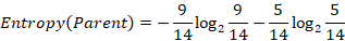
· Calculate the impurity for the initial training data set.
We have four male and three female so the entropy is equal to:
· Calculate the information gain for the “Age” attribute
The age attribute has two distinct values, which are young and adult, the first step before calculating the information gain. We should calculate the impurity for each value.
Calculate the entropy for the “Young” value of the “Age” attribute:


Calculate the entropy for the “adult” value of the “age” attribute:


The information gain for the “age” attribute is equal to:


Calculate the information gain for the “weight” attribute.


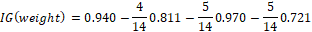

Calculate the information gain for the “length” attribute.


The Table 3 summarizes all the result that we get above.
Table 3. Information gain by ID3| Age | Weight | Length | |
| Information Gain | 0.102 | 0.104 | 0.247 |
The length attribute returns the maximum information gain, so the ID3 algorithm will split the initial records based on the values of this attribute. Each value will be the outcome of the root node. Length attribute will produce three outcomes, short, medium and long. The splitting will therefore also produce three sub-sets. Each sub set has the records that the value of the “length” attribute will match the value of the outcome. The ID3 algorithm will create the first root node (Figure 6 a) and its outcomes as described below:
Figure 6a.The root node of the decision tree.
In the outcome associated with the “short” value the class label has the same value for all the records. Therefore, the ID3 will end in this child node and will create a leaf node that has the value “female”, but for the others child nodes, the stopping conditions are not verified, the algorithm will repeat the process until reaching a homogenous sub node. At the end of the process, the ID3 algorithm generate a tree model as shown below.
The root node and the intern nodes are in green, the leaf nodes are in red, and the outcomes are in orange.
In general, decision tree represents a disjunction of conjunctions on the attribute values of records. Each path from the tree root to the leaf node corresponds to a conjunction of attribute test. In addition, the tree itself to a disjunction of these conjunctions. For example, the decision tree shown in Figure 7 corresponds to the expression
Figure 7.The full decision tree model.


The above disjunctions of conjunctions can be used as a function to predict new records with unknown class label “gender”. Thus, each disjunction become an “If” statement and each conjunction become a condition for testing the value of each attribute of the new record. We will generate five rules from this decision tree model to predict new records as shown below.
Model_to_Rules(New_Record)
if new_record(Length) = ”Short” then
return female
else if new_record(Length) = “Medium” AND new_record(weight) = Middle OR
new_record (weight) = Light then
return female
else if new_record(Length) = “Medium” AND new_record(weight)= Heavy then
return male
else if new_record(Length) = “Long” AND new_record(weight) = “Light” OR new_record(weight) = “Heavy” then
return female
else if new_record(Length) = “Long” AND new_record(weight) = “Middle” then
return male
Limitation of ID3 Algorithm
In the real world data, the dataset can contain different types of data. Such as Boolean data, categorical data and continues data. In this section we will work with the previous training data set, but with a small difference, the weight attribute will be defined by continues values instead of categorical values, in order to see how the ID3 will react to this small difference, and try to understand the limitation of the ID3 to numeric data. The table below (Table 4) show the training data set with two categorical attributes (age and length); one continues attribute (weight) and a class label (gender).
Table 4. The initial training data set.| Age | Weight | Length | Gender |
|---|---|---|---|
| Young | 72 | Long | male |
| Adult | 52 | Short | female |
| Young | 92 | Medium | male |
| Adult | 76 | Long | female |
| Adult | 70 | Short | female |
| Young | 67 | Medium | male |
| Young | 60 | Medium | female |
| Adult | 62 | Long | male |
| Adult | 74 | Short | female |
| Young | 58 | Medium | female |
| Adult | 59 | Medium | female |
| Adult | 75 | Short | female |
| Adult | 71 | Long | male |
| Adult | 61 | Long | female |
The process is the same, the goal is to build a decision tree model, the ID3 algorithm need to calculate the information gain for each attribute as a first step, the values for the age and length attributes still the same, because we do not change the values for this two attributes, the only difference is about the weight attribute.
· Information gain for the “Age” attribute is equal to:
· Information gain for the “Length” attribute is equal to:
· Calculate the information gain for the “Weigh” attribute:
Before calculating the information gain, we must first calculate the impurity for each possible value of the “weight” attribute, the weight attribute producing fourteen values, each value linked to a single record, so that the entropy for each value will be zero. Here is an example of the value “72”, its entropy equal to:
While the entropy for all the values is null, so the information gain of the “weight” attribute is equal to the entropy of the initial dataset:


We can recognize without calculation, that the “weight” attribute will produce the highest entropy, because the weight attribute will generate fourteen purer subsets, each subset has only one record belongs to one class. The ID3 will end here because there are no more records to split and all the sub-sets are homogenous. The decision tree model generated is shown in Figure 8.
Figure 8.Decision tree model generated by ID3 with numeric attribute.
The above training dataset has only one numeric attribute, and the ID3 algorithm fails to generate a model that will generally predict new future records. The ID3 algorithms is less effective for numeric attributes, with a training dataset that has more than one numeric attribute and noisy and missing data, the ID3 algorithm is bad choice. The better solution for this type of datasets is the C4.5 algorithm, which we will discover in the next section.
C4.5 Learning Algorithm
C4.5 is evolution of ID3, presented by the same author (Quinlan, 1993). The C4.5 algorithm generates a decision tree for a given dataset by recursively splitting the records. The C4.5 algorithm considers the categorical and numeric attributes. For each categorical attribute, the C4.5 calculate the information gain and select the one with the highest value, and used the attribute to produce many outcomes as the number of distinct values of this attribute 8, 9, 10. For each numeric attribute there are two methods to calculate the information gain, the first method consists in calculating the gain ratio, and the second method consists in calculating the information gain as we did in the ID3 but with some differences.
As an example, we take the training dataset that we already used in the ID3 limitation section.
Calculations of categorical attributes do not change. The C4.5 uses the same process as ID3 to calculate the categorical attribute. The main difference between ID3 and C4.5 concerns numeric attributes, C4.5 presents two methods for managing the numeric values of an attribute. The information gain of categorical values is still the same as we did before.
First method
What is the wrong with the “weight” attribute? Simply, it has so many possible values that is used to separate the training records into very small sub-sets. Because of this, the weight attribute will have the highest information gain relative to the initial training dataset. Thus, the resulting model will be a very poor predictor of the target class label over new future records.
One way to avoid this difficulty is to select decision attributes based on some measure other than information gain. One alternative measure that has been used successfully is the gain ratio. The gain ratio measure penalizes attributes penalizes attributes such as weight attribute by incorporating a term called split information 11, that is sensitive to how uniformly the attribute split the data:

Where c is the total number of splits, and p(vj) is the fraction of the records associated with a split by the total number of all the records. For an example, the weight attribute has fourteen possible values, so the number of splits c in this example is equal to fourteen, and the number of records associated to each possible value is equal to one, each attribute value has the same number of records then:

Where N(vj) the number of records is associated with a split or an unique value, and N is the total number of records.

Each attribute value has the same number of records, so the split info will be equal to:

To determine the goodness of a split, we need to use a criterion known as gain ratio. This criterion is defined as follows:

The information gain of the weight attribute is equal to the entropy of the initial data set, we have been discussed this topic previously in the fifth section. The gain ratio of the weight attribute is equal to:

This example suggests that if an attribute produces large number of splits, its split information will also be large, which in turn reduces its gain ratio.
The information gain for all the attributes is given in Table 5.
Table 5. Information Gain| Age | Weight | Length | |
| Information Gain | 0.102 | 0.246 | 0.247 |
Using this first technique in C4.5, the attribute “length” always provides the great information gain than the attributes “age” and “weight”.
· Second method
This method consists in considering each value of a numeric attribute as a candidate, then for each candidate (numeric value) select the set of records less than or equal to this candidate, and the set of records greater than this candidate. In addition, calculate the entropy for the two sets, and the information gain for the candidate that relates to the two sets of records 7. Here is a full example (Table 4) of how we use this method on the weight attribute. For example, consider the candidate who has the value “61”. This candidate can divide the initial training dataset into two sub-sets, the first subset with the records whose weight value is less than or equal to “61”, and the second sub-set with the records whose weight value is greater than “61”. The calculation of entropy and information gain are presented in Table 6.
Table 6. Calculations for each value of weight attribute| classes | Entropy | Gain | |||
| male | female | ||||
| 52 | <= | 0 | 1 | 0 | 0.0197 |
| > | 5 | 8 | 0.991 | ||
| 58 | <= | 0 | 2 | 0 | 0.100 |
| > | 5 | 7 | 0.979 | ||
| 59 | <= | 0 | 3 | 0 | 0.159 |
| > | 5 | 6 | 0.994 | ||
| 60 | <= | 0 | 4 | 0 | 0.225 |
| > | 5 | 5 | 1 | ||
| 61 | <= | 0 | 5 | 0 | 0.302 |
| > | 5 | 4 | 0.991 | ||
| 62 | <= | 1 | 5 | 0.650 | 0.09 |
| > | 4 | 4 | 1 | ||
| 67 | <= | 2 | 5 | 0.863 | 0.016 |
| > | 3 | 4 | 0.985 | ||
| 70 | <= | 2 | 6 | 0.811 | 0.048 |
| > | 3 | 3 | 1 | ||
| 71 | <= | 3 | 6 | 0.918 | 0.0034 |
| > | 2 | 3 | 0.970 | ||
| 72 | <= | 4 | 6 | 0.970 | 0.015 |
| > | 1 | 3 | 0.811 | ||
| 74 | <= | 4 | 7 | 0.945 | 0.00078 |
| > | 1 | 2 | 0.918 | ||
| 75 | <= | 4 | 8 | 0.918 | 0.0102 |
| > | 1 | 1 | 1 | ||
| 76 | <= | 4 | 9 | 0.890 | 0.113 |
| > | 1 | 0 | 0 | ||
| 92 | <= | 5 | 9 | 0.940 | 0 |
| > | 0 | 0 | 0 | ||


The information gain of the value”61” will be the information gain of the weight attribute (Table 7).
Table 7. Information gain| Age | Weight | Length | |
| Information Gain | 0.102 | 0.302 | 0.247 |
C4.5 will split the records into two sub-sets, the first subset with records whose weight value is less than or equal to “61”, the second subset with records whose weight value is greater than “61”.
· The first subset (Table 8)
Table 8. Same class label| Age | Length | Gender |
|---|---|---|
| Adult | Short | female |
| Young | Medium | female |
| Young | Medium | female |
| Adult | Medium | female |
| Adult | Long | female |
All of the records in this subset have the same class label, so the subset is homogenous, the C4.5 will end at this node and create a leaf node with the value “female”.
· The second subset.
This second subset is heterogeneous (Table 9), so the C4.5 algorithm repeats the process until reaching homogenous subsets.
Table 9. Heterogeneous class label| Age | Length | Gender |
|---|---|---|
| Young | Long | male |
| Young | Medium | male |
| Adult | Long | female |
| Adult | Short | female |
| Young | Medium | male |
| Adult | Long | male |
| Adult | Short | female |
| Adult | Short | female |
| Adult | Long | male |
The C4.5 algorithm has many advantages over ID3 algorithm 9. One of the main advantages is to manage both continues and categorical attributes, for the continues attribute and as we saw above, the C4.5 creates a threshold, then divides the initial records into those whose attribute value is greater than the threshold and those that are less than or equal to it. The other advantages are:
Þ Handling training data set with missing values, the real data set is not perfect. They may have noisy and missing values.
Þ Pruning trees after creation means that C4.5 will remove branches from the tree that are repeated or unnecessary, by replacing them with a leaf node.
Conclusion
In this article, we explain entropy and information gain measures, we discussed the usefulness and the importance of these measures and how they were used in the decision tree algorithm to build a model that will be used later for prediction. This article also gives an overview of the ID3 and C4.5 algorithms, and explain how they work. In future work we will use these algorithms for classification project.
References
- 1.A S Fitrani, M A Rosid, Findawati Y, Rahmawati Y, Anam A K. (2019) Implementation of ID3 algorithm classification using web based weka,The. 1st International Conference on Engineering and Applied Science, Journal of Physics: Conference Series.IOP Publishing,doi;10.1088/1742-6596/1381/1/012036 1381-012036.
- 2.Wang Yingying, Li Yibin, Song Yong, Rong Xuewen, Zhang Shuaishuai. (2017) . Improvement of ID3 Algorithm Based on Simplified Information Entropy and Coordination Degree, Algorithms.doi: 10.3390/a10040124.www.mdpi.com/journal/algorithms 10-124.
- 3.Sharma Seema, Agrawal Jitendra, Sharma Sanjeev. (2013) Classification through Machine Learning Technique: C4.5 Algorithm based on Various Entropies. , International Journal of Computer Applications(0975-8887)82(16)November2013
- 4.Sudrajat R, Irianingsih I, Krisnawan D. (2017) Analysis of data mining classification by comparison of. C4.5 and ID algorithms, IORA IOP Publishing, IOP Conf. Series: Materials Science and Engineering.doi;10.1088/1757-899X/166/1/012031 166-012031.
- 5.Setiawan K Mukiman H, S Hanadwiputra. (2019) A Suwarno, C4.5 Classification Algorithm Based On Particle Swarm Optimization To Determine The Delay Order Production Pattern. INCITEST 2019, IOP Conf. Series: Materials Science and Engineering.IOP Publishing.doi: 10-1088.
- 6.Sinam I, Lawan Abdulwahab.An Improved C4.5 Model Classification Algorithm Based On Taylor’s Series. , Jordanian Journal of Computers and Information Technology(JJCIT),April2019 5(1).
- 8.Singh Sonia, Gupta Priyanka. (2014) Comparative Study ID3, CART, and C4.5 Decision Tree Algorithm: a survey”. International Journal of Advanced Information Science and Technology, Vol27, No.27, pp-99 .
- 9.Kumar Sunil, Sharma Himani. (2016) A Survey on Decision Tree Algorithms of Classification in. Data Mining”, International Journal of Science and Research, Vol-5 Issue4 2094-2095.
Cited by (1)
- 1.Forghani Ebrahim, Sheikh Reza, Hosseini Seyed Mohammad Hassan, Sana Shib Sankar, 2022, The impact of digital marketing strategies on customer’s buying behavior in online shopping using the rough set theory, International Journal of System Assurance Engineering and Management, 13(2), 625, 10.1007/s13198-021-01315-4